
3D FEM Simulation
Bethany Witemeyer
Overall Idea
For this project, I wrote a three-dimensional, volumetric FEM simulator. This simulator uses a stable neo-Hookean material model, and it can simulate both objects falling under gravity and objects being acted upon by pulling forces. The simulator also has an "offline" mode where the simulation can be run without rendering the scene. Finally, as the mesh size increases, the time needed to run the simulation increases. To combat this, I have implemented a method called "freezing the Jacobian."

Bunny mesh falling under gravity
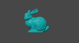
Bunny mesh in rest position

Bunny mesh being pulled by the nose
Animation Techniques
Physically-Based Animation - 3D FEM
The simulator uses 3D FEM to simulate the motion of a volumetric mesh. The mesh is represented by nodes and tetrahedra. For each step of the simulation, we must solve the following equation:
In the above equations, K is the stiffness matrix and is dependent on the material model used in the simulation. This simulator uses the stable neo-Hookean material model.
Physically Based Animation - Forces
The simulator has support for two types of forces: gravity and pulling forces. Gravity is always present in the simulation. When the simulation is not being run in "offline" mode, the user can use key bindings to change the direction and magnitude of gravity.
The second type of force supported by the simulator is pulling forces. These forces are spring forces applied to a single node in the mesh for a specified amount of time. However, these forces can very easily cause the simulation to become unstable. To increase the stability of the simulation, the force is also applied to the nodes surrounding the main node. However, the magnitude of the force applied to the surrounding nodes decreases linearly as the distance from the main node increases. Another technique used to stabilize these forces is to linearly interpolate the distance the spring is stretched using time. This ensures that the force doesn't change the simulation too quickly.
Libraries/Packages
Eigen
Eigen was used for the matrix operations in the simulator, as well as for interfacing with CHOLMOD's solver.
CHOLMOD
Written by Dr. Tim Davis, CHOLMOD uses the Cholesky factorization to solve systems of linear equations. It has been optimized for sparse matrices, and was used to help increase the speed of the simulator.
Brender
Developed by Dr. Sudea et al., brender provides a simple way to export a simulation and load it into blender. This was used in the "offline" mode of the simulator. As the simulations were often very slow, this was a very helpful tool in visualizing the simulations.
Stable Neo-Hookean
This material model was developed by Dr. Ted Kim. It is the material model used for the deformable objects in the simulations.
TetGen
TetGen is software developed by Hang Si for generating volumetric meshes. Nick Weider was a big help in using this software to generate the meshes used in the simulations.
Speeding Up the Simulation
3D FEM simulation can be very slow for larger meshes. This is due to expensive calculations that happen each time step. One of these calculations is for the stiffness matrix K. Another is computing the Cholesky factorization of A. One option for reducing this cost is not to calculate A every time step. Instead, we store the factorization of A and use it for the next x steps (step limit in the videos below). To keep the simulation accurate, we need to recalculate A occasionally, and we must always recalculate b. However, on the steps that we use a previous value of A, we don't need to calculate K and we don't need to factorize A. Thus, those steps are significantly cheaper than the steps when A is calculated. This method is called "freezing the Jacobian."
Normal
Step Limit = 5
Step Limit = 10
Step Limit = 20
As seen in the videos above, increasing the number of skipped steps results in simulations that look relatively the same. However, when we look at the time it takes for each simulation to run, we see that skipping steps and using a previous value for A results in a much faster simulation. These results can be seen in the graph below.
